Join functionality
Applies to: CELONIS 4.0 CELONIS 4.2 CELONIS 4.3 CELONIS 4.4 CELONIS 4.5 CELONIS 4.6 CELONIS 4.7
Description
Celonis performs implicit joins when a query accesses several tables. This means that the user does not have to define the join as part of a query, but the tables are joined as defined in the Data Model Editor.
Implicit joins
[1] Here ActivityTable and CaseTable are queried. The customer information of the CaseTable is implicitly joined to the activities of the ActivityTable:
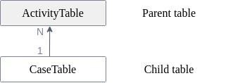 |
Joins are always done as outer left equi join. In this example the ActivityTable is on the left side of the join. Therefore the activity D which doesn't have a join partner in the case table, is part of the result, while Case ID 4 is not. Also it is noteworthy that null values are never joined, as it is the case for activity E.
Which table is on the left side of the join, depends on the join cardinality. Celonis supports 1 - N relations. 1 - N relation means that if for example Table A and B are joined together, every row in B can have zero or one join partner in table A but not more. The other way around there is no limitation. Every row in A can have an arbitrary number of join partners. This sounds maybe limiting but 1 - N join can actually also process N - 1 and 1 - 1 relations. N - 1 relations will be simply turned around to 1 - N relations by Celonis. A 1 - 1 relation is only a special case of a 1 - N relation. But N - M joins are not supported because they are rare, can be transformed into simpler relations and make it much harder to understand the result.
The N side is always put on the left side of the join. In this example, it is easy to see that case 1 and 2 have two join partners in the activity table, while every activity relates to exactly one case. Therefore the ActivityTable is on the left side of the join.
In other words ActivityTable is the fact table (Parent), and CaseTable is the dimension table (Child). These terms are explained in more detail below.
|
Parent and Child tables
Not every table can be joined to every other table within one data model. To understand which tables can be joined together one has to know that Celonis supports an extended Snowflake schema for a data model. A Snowflake schema consists of one fact table which can have multiple N - 1 relations to dimension tables. These dimension tables can themselves have N - 1 relations to other tables. Celonis extends the classic Snowflake schema by supporting multiple fact tables but no cyclic join graphs. To resolve a cyclic join graph you may have to add a table multiple times to the data model.
We categorize the tables in Parent tables and Child tables. The term becomes clear if a schema is interpreted as a family tree where the fact table is the root as can be seen in the following example:
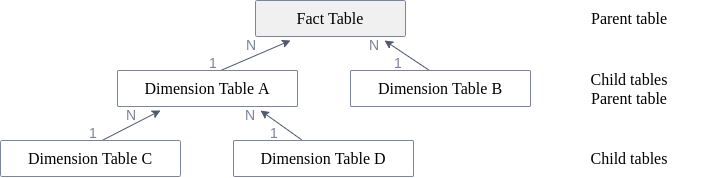 |
For Dimension Table A and Dimension Table B the Fact Table is the parent table. For Dimension Table C and Dimension Table D the Dimension Table A is the common parent table and the Fact Table the grand parent table. To process a join Celonis first identifies the closest common ancestor. For example if a column from Dimension Table A should be joined with a column from Dimension Table B, Celonis identifies the Fact Table as closest common parent. It then joins the needed columns from Dimension Table A and Dimension Table B to the Fact Table. We call this step pulling up the data. The closest common ancestor does not always have to be the Fact Table. It also can be another dimension table like for Dimension Table C and Dimension Table D for which Dimension Table A is the closest common ancestor.
This works perfectly as long as you have only one fact table. If you have multiple fact tables it might not be possible to identify a common ancestor for your join. To get a better understanding of the issue we look at the following schema:
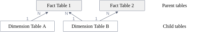 |
Dimension Table A and Dimension Table B still can be joined. Dimension Table B can be joined with Fact Table 1 and also with Fact Table 2.
Understanding the "No common parent" error message
Dimension Table A can not be joined with Fact Table 2. Also the two fact tables can not be joined and would result in the following error:
Warning
No common parent between tables could be found - please check your schema. The tables Fact Table 1 and Fact Table 2 are connected, but have no common parent table. For more information on the following join path, search for "Join functionality" in PQL documentation: [Fact Table 1]N <-- 1![Dimension Table B]!1 --> N[Fact Table 2]
As mentioned, the join graph is acyclic, which means there is exactly one join path between any two connected tables. In case of no common parent between two connected tables, the join path is also shown in the error message (see above). The join path contains the following information:
Table name:
[Fact Table 1]A table surrounded by exclamation marks breaks the possibility of a common parent:
![Dimension Table B]!Join direction:
-->or<--Join cardinalities:
1 --> NorN <-- 1