SOURCE - TARGET
Applies to: CELONIS 4.0 CELONIS 4.2 CELONIS 4.3 CELONIS 4.4 CELONIS 4.5 CELONIS 4.6 CELONIS 4.7
Description
SOURCE and TARGET functions provide a way to combine values from two different rows of the activity table into the same row, e.g. for calculating the throughput time between consecutive events inside a case.
In process mining applications it is often required to relate an event to another event which directly or eventually follows. For instance, this is required to compute the throughput time between two events by calculating the difference between the corresponding timestamps. Due to the relational data model, the timestamp values to subtract are stored in different rows. However, the operators (e.g. arithmetic operations) usually can only combine values from the same row. Therefore, we need a way to combine values from two different rows into the same row for performing such computations.
To overcome this issue, PQL relies on the SOURCE and TARGET operators.
Syntax
Adds the values from a column, which correspond to a source activity, to a temporary table based on the optional filter column and the optional edge configuration:
SOURCE ( activity_table.column [, activity_table.filter_column ] [, edge_configuration ] )
Adds the values from a column, which correspond to a target activity, to a temporary table based on the optional filter column and the optional edge configuration:
TARGET ( activity_table.column [, activity_table.filter_column ] [, edge_configuration ] )
activity_table.column: Column of the activity table. Its values are mapped to the referred events and returned as result column. The result column is stored in a temporary result table which can be joined with the case table.
activity_table.filter_column: Optional filter column to skip certain events. Events with a NULL value in the related entry of the filter column are ignored. Usually, the filter column is created using REMAP_VALUES. See below for detailed explanation.
edge_configuration: Describes which edges between the activities of a case are considered. Must be one of:
ANY_OCCURRENCE[] TO ANY_OCCURRENCE[] (DEFAULT)
FIRST_OCCURRENCE[] TO ANY_OCCURRENCE[]
FIRST_OCCURRENCE[] TO ANY_OCCURRENCE_WITH_SELF[]
ANY_OCCURRENCE[] TO LAST_OCCURRENCE[]
FIRST_OCCURRENCE[] TO LAST_OCCURRENCE[]
See below for detailed explanation.
The following example illustrates how SOURCE and TARGET can be used to compute the throughput time between an event and its direct successor. While SOURCE always refers to the actual event, TARGET refers to its following event inside the case. Such a connection is called an edge. Consequently, SOURCE and TARGET can be used to combine an event with its following event in the same row of a table. Both operators accept a column of the activity table as input and return the respective value of the referred event, as illustrated in the following example.
Besides the computation of custom process KPIs, like the throughput time between certain activities, SOURCE and TARGET also enable more advanced use cases, like the Segregation of Duties.
[1] For the first event in the Activities table, The example also demonstrates how the
|
NULL handling
Rows from activity_table.column, which are NULL, are also NULL in the output column. The SOURCE / TARGET operators ignore rows in which the value of the filter column are NULL.
Filter Column
To skip certain events, the SOURCE and TARGET operators accept an optional filter column as a parameter. This column must be of the same size as the activity table. The SOURCE and TARGET operators ignore all events that have a NULL value in the related entry of the filter column. Usually, the filter column is created using the REMAP_VALUES operator.
[2] This example query returns the activity names of the source and target events given in the input activity table. However, the result table only shows one row relating 'A' to 'D' because the activities 'B' and 'C' are filtered out. This is achieved by passing the result of the REMAP_VALUES operator to the
|
Edge Configurations
To define which relationships between the events should be considered, the operators offer the optional edge configuration parameter. The following edge configuration options are available:
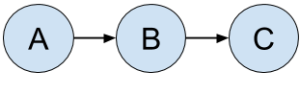 |
(a) ANY_OCCURRENCE[] TO ANY_OCCURRENCE[] (DEFAULT)
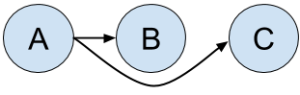 |
(b) FIRST_OCCURRENCE[] TO ANY_OCCURRENCE[]
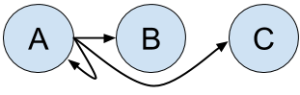 |
(c) FIRST_OCCURRENCE[] TO ANY_OCCURRENCE_WITH_SELF[]
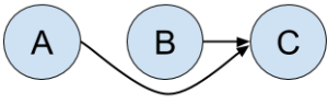 |
(d) ANY_OCCURRENCE[] TO LAST_OCCURRENCE[]
 |
(e) FIRST_OCCURRENCE[] TO LAST_OCCURRENCE[]
The first option (a) is the default and only considers the direct follow relationships between the events, while option (b) only considers relationships from the first event to all subsequent events. Option (c) is similar to option (b) but also considers self-loops of the first event. Option (d) is the opposite of option (b) and only considers relationships going from any event to the last event. Finally, option (e) only considers the relationship between the first and the last event. The different options enable the user to compute KPIs between different activities of the process. For example, you can use option (b) to compute how many minutes after the start of the process (indicated by the first activity 'A') an activity was executed. This is illustrated in the following example:
[3]
|
Configuration Propagation
To simplify the query, the optional edge configuration and the filter column need to be defined in only one occurrence of SOURCE or TARGET per query. The settings are implicitly propagated to all other operators in the same query. This can be seen in the examples above, where all SOURCE and TARGET occurrences inherit the filter column or the edge configuration from the first SOURCE operator of the query.
Join behavior
SOURCE and TARGET generate temporary edge tables. A separate edge table is created for each unique edge and filter column configuration inside a query. SOURCE and TARGET operators with identical edge configuration and filter column add columns to the same edge table. The edge tables are joined to the corresponding case table.
Example
In this example several calls to the SOURCE and TARGET operators are done. After each call the status of the edge tables is shown.
SOURCE ( Activity, ANY_OCCURRENCE[] TO ANY_OCCURRENCE[] )
SOURCEis called with theANY_OCCURRENCE[] TO ANY_OCCURRENCE[]edge configuration. A temporary edge table is created and theSOURCEcolumn is added to it: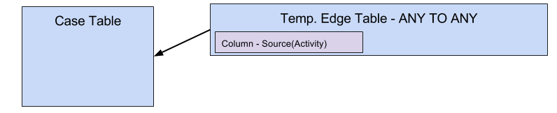
TARGET ( Activity, ANY_OCCURRENCE[] TO ANY_OCCURRENCE[] )
TARGETis also called with theANY_OCCURRENCE[] TO ANY_OCCURRENCE[]edge configuration. As this is the same configuration as in the previousSOURCEcall, theTARGETcolumn is added to the existing edge table: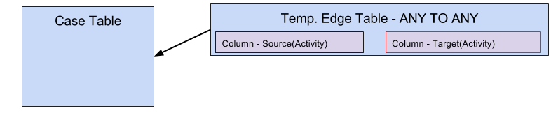
This column is added to a new temporary table, because the configuration is different to the previous ones:
SOURCE ( Activity, Filter, ANY_OCCURRENCE[] TO ANY_OCCURRENCE[] )
SOURCEis called with a filter column configuration. TheFiltercould be a call to REMAP_VALUES as shown above. Although the edge configurationANY_OCCURRENCE[] TO ANY_OCCURRENCE[]is the same as in the calls before, the overall configuration differs because of the additional filter column. Therefore, a new temporary edge table is created, and theSOURCEcolumn is added to it: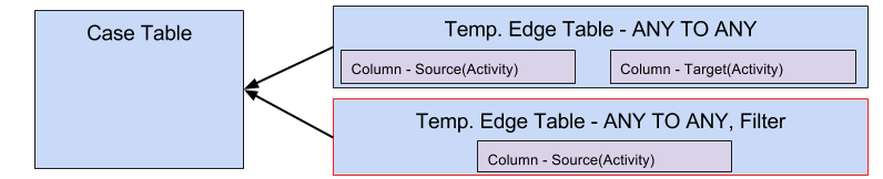
Multiple temporary edge tables can lead to problems if used within the same query. This happens if SOURCE and TARGET operators with different edge and filter configurations are used within the same query. The edge tables cannot be joined together by default because they do not have a common parent. This behavior is described in Join functionality in more detail.
The only way of having multiple different configurations inside the same query is to aggregate values of the temporary edge tables to the case table using PU functions, as shown in the following example:
[4] This example shows how two different configurations can be used inside one query. For each case, we can calculate the average number of minutes between consecutive activities. Result Column2 shows the result when ignoring activity 'A' for the calculation using the corresponding filter configuration, and Result Column3 shows the result when ignoring activity 'B'. In both cases, the number of minutes between corresponding
|
Filter behavior
As described above, the temporary edge tables are joined to the case table. This means that if a case is filtered out in the case table, all activities related to that case in the temporary edge tables are also filtered out. This also holds vice versa: if all activities related to a case are filtered out in the edge table, the case itself is also filtered out in the case table. If not all edges of a case are filtered out, the case stays in the case table. Filter Propagation describes the filter propagation behavior in more detail.
[5] In this example, we filter based on the temporary edge table. The filter only keeps edges where the
|